Sample Size (1)

library(pwr)
library(WebPower)
Loading required package: MASS

Attaching package: 'MASS'
The following object is masked from 'package:dplyr':

    select
Loading required package: lme4
Loading required package: Matrix

Attaching package: 'Matrix'
The following objects are masked from 'package:tidyr':

    expand, pack, unpack
Loading required package: lavaan
This is lavaan 0.6-16
lavaan is FREE software! Please report any bugs.
Loading required package: parallel
Loading required package: PearsonDS
library(simstudy)

Overview

Packages for Sample Size

Functions & packages for Sample Size

Typical Values

  • A two-tailed test

  • a significance of 0.05 and a power of 80% was established.

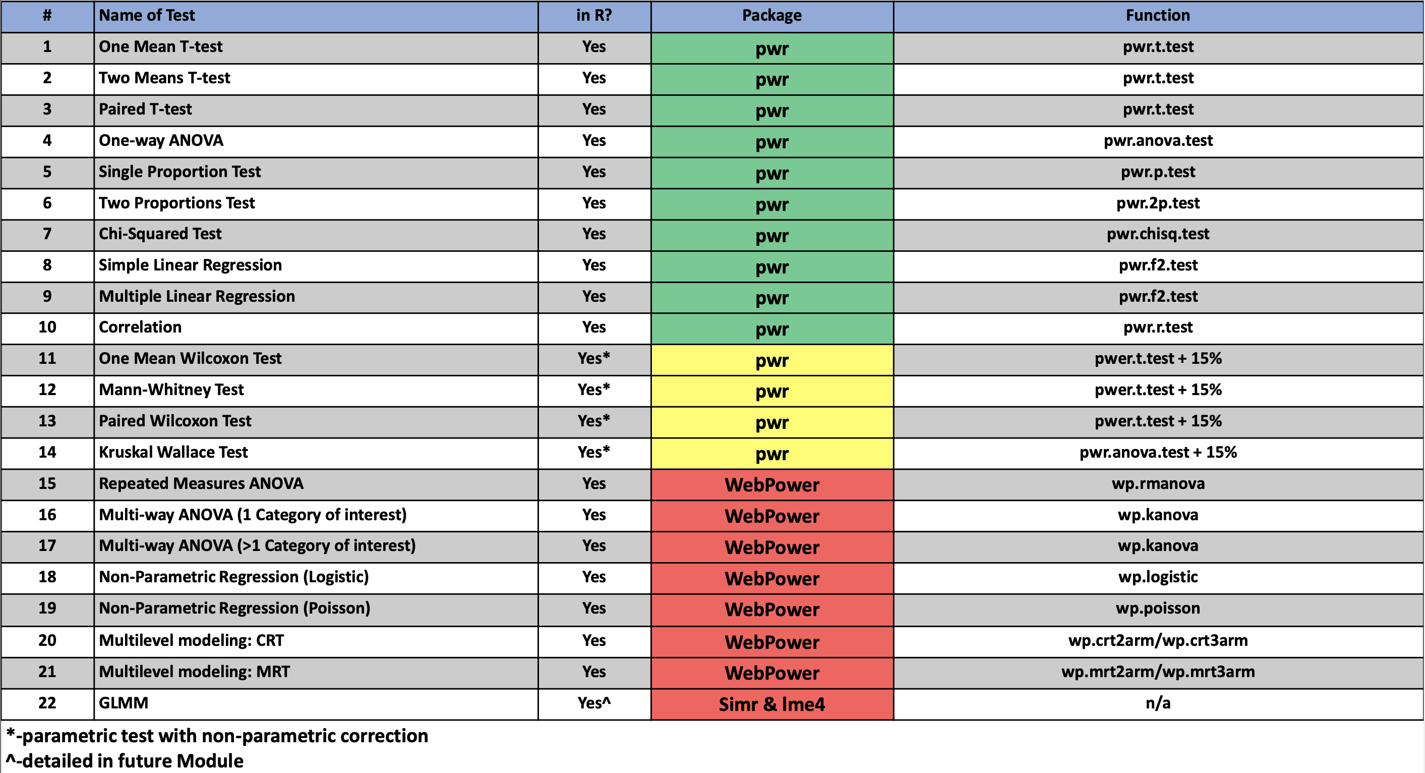
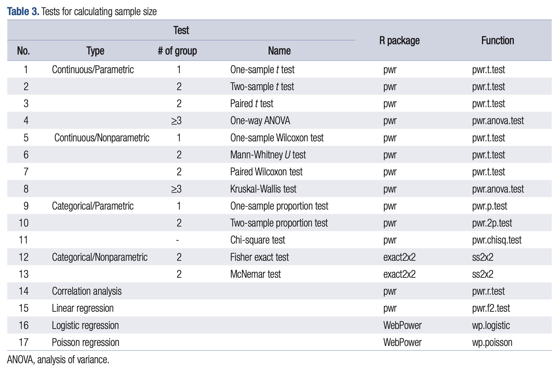
  • For nonparametric tests on continuous variables, as a rule of thumb, calculate the sample size required for parametric tests and add 15%

Effect Size

  • Effect size can be defined as ‘a standardized measure of the magnitude of the mean difference or relationship between study groups’

  • An index that divides the effect size by its dispersion (standard deviation, etc.) is not affected by the measurement unit and can be used regardless of the unit, and is called an ‘effect size index’ or ’standardized effect size

  • Whether an effect size should be interpreted as small, medium, or large may depend on the analysis method.

  • We use the guidelines mentioned by Cohen and Sawilowsky and use the medium effect size considered for each test in the examples below.

Conventional Effect Size

cohen.ES(test = "t", size = "medium")

     Conventional effect size from Cohen (1982) 

           test = t
           size = medium
    effect.size = 0.5

Two Means T-test

tests if a mean from one group is different from the mean of another group for a normally distributed variable. AKA, testing to see if the difference in means is different from zero.

Effect size for t-test: 0.2 = small, 0.5 = medium, 0.8 = large effect sizes

\[ d = \frac{\mu_1 - \mu_2}{s_{pooled}} \] The pooled standard deviation ( \(s_{pooled}\) ) is calculated as:

\[ s\_{pooled} = \sqrt{\frac{(n_1 - 1)s_1^2 + (n_2 - 1)s_2^2}{n_1 + n_2 - 2}} \] ### Ex 1: Caloric Intake

Find N

You are interested in determining if the average daily caloric intake different between men and women. You collected trial data and found the:

  • average caloric intake for males to be 2350.2 (SD=258)
  • females had intake of 1872.4 (SD=420).

(Don’t know N for each group)

sd_pooled_1 <- sqrt((258^2 + 420^2)/2)
sd_pooled_1
[1] 348.5427
eff_size1 <- (2350.2 - 1872.4) / sd_pooled_1
eff_size1
[1] 1.370851
pwr.t.test(d = eff_size1, 
           sig.level=0.05, 
           power=0.80, type= "two.sample", alternative="two.sided")

     Two-sample t test power calculation 

              n = 9.417703
              d = 1.370851
      sig.level = 0.05
          power = 0.8
    alternative = two.sided

NOTE: n is number in *each* group

Simulate

def_1 <- simstudy::defData(
  varname = "intake_male", formula = 2350.2,
  variance = 258^2
) |>
  simstudy::defData(
    varname = "intake_female", formula = 1872.4,
    variance = 420^2
  )

set.seed(123)
df_intake <- genData(n = 10, def_1) |> 
  pivot_longer(cols = starts_with("intake"), names_to = "gender", 
               values_to = "intake", names_prefix = "intake_") |> 
  dplyr::select(-id)

df_intake |> 
  group_by(gender) |> 
  rstatix::get_summary_stats(type = "mean_sd")
# A tibble: 2 × 5
  gender variable     n  mean    sd
  <chr>  <fct>    <dbl> <dbl> <dbl>
1 female intake      10 1960.  436.
2 male   intake      10 2369.  246.
rstatix::t_test(df_intake, intake ~ gender) # Sig
# A tibble: 1 × 8
  .y.    group1 group2    n1    n2 statistic    df      p
* <chr>  <chr>  <chr>  <int> <int>     <dbl> <dbl>  <dbl>
1 intake female male      10    10     -2.59  14.2 0.0214

Ex 2

You are interested in determining if the average protein level in blood different between men and women. You collected the following trial data on protein level (grams/deciliter).

prot_samp <- data.frame(
  gender = c(rep("M", 8), rep("F", 8)),
  prot = c(
    c(1.8, 5.8, 7.1, 4.6, 5.5, 2.4, 8.3, 1.2), # Male
    c(9.5, 2.6, 3.7, 4.7, 6.4, 8.4, 3.1, 1.4) # Female
  )
)
prot_samp |> 
  group_by(gender) |> 
  summarise(mean = mean(prot), sd = sd(prot))
# A tibble: 2 × 3
  gender  mean    sd
  <chr>  <dbl> <dbl>
1 F       4.98  2.88
2 M       4.59  2.58
eff_size2 <- (4.9750 - 4.5875   ) / sqrt((2.875388^2 + 2.575399^2) / 2)
eff_size2
[1] 0.1419665
pwr.t.test(d = eff_size2, sig.level=0.05, 
           power=0.80, type= "two.sample", alternative="two.sided")

     Two-sample t test power calculation 

              n = 779.8317
              d = 0.1419665
      sig.level = 0.05
          power = 0.8
    alternative = two.sided

NOTE: n is number in *each* group

ANOVA

Effect Size of ANOVA (f)

Partial Eta Squared (η2) = SStreat / SStotal
f = √((η2 /(1- η2)

Total Sum of Squares (SStotal):

\[ \text{SStotal} = \sum (Y_i - \bar{Y})^2 \]

where ( \(Y_i\) ) are the individual data points and ( \(\bar{Y}\) ) is the overall mean.

Treatment Sum of Squares (SStreat):

\[ \text{SStreat} = \sum n_j (\bar{Y}_j - \bar{Y})^2 \]

where ( \(n_j\) ) is the number of observations in each group, ( \(\bar{Y}_j\) ) is the mean of each group, and ( \(\bar{Y}\) ) is the overall mean.

Ex 1: Sx Option

You are interested in determining there is a difference in weight lost between 4 different surgery options. You collect the following trial data of weight lost in pounds

sx_opt <- data.frame(
  op1 = c(6.3, 2.8, 7.8, 7.9, 4.9),
  op2 = c(9.9, 4.1, 3.9, 6.3, 6.9),
  op3 = c(5.1, 2.9, 3.6, 5.7, 4.5),
  op4 = c(1, 2.8, 4.8, 3.9, 1.6)
) |> 
  pivot_longer(cols = everything(), names_to = "op", values_to = "wt_loss")
sx_opt_aov <- aov(wt_loss ~ op, data = sx_opt)
sx_opt_aov_tbl <- summary(sx_opt_aov)
sx_opt_aov_tbl
            Df Sum Sq Mean Sq F value Pr(>F)  
op           3  37.13  12.375    3.46 0.0414 *
Residuals   16  57.22   3.576                 
---
Signif. codes:  0 '***' 0.001 '**' 0.01 '*' 0.05 '.' 0.1 ' ' 1

SStreat

\[ \text{SStreat} = \sum n_j (\bar{Y}_j - \bar{Y})^2 \]

SStreat <- sx_opt_aov_tbl[[1]]["op", "Sum Sq"]
SStreat
[1] 37.1255

Or

sx_opt |> 
  group_by(op) |> 
  summarise(mean_gr = mean(wt_loss), n = n()) |> 
  mutate(SStx_gr = n * (mean_gr - mean(sx_opt$wt_loss))^2) |> 
  summarise(SStx = sum(SStx_gr))
# A tibble: 1 × 1
   SStx
  <dbl>
1  37.1

SStotal

SStotal <- sum((sx_opt$wt_loss - mean(sx_opt$wt_loss))^2)
SStotal
[1] 94.3455

Or

SStotal <- sum(sx_opt_aov_tbl[[1]][, "Sum Sq"])
SStotal
[1] 94.3455

Effect Size (f)

Partial Eta Squared (η2) = SStreat / SStotal
f = √((η2 /(1- η2)
n_squared <- SStreat / SStotal
eff_size3 <- sqrt(n_squared / (1 - n_squared))
eff_size3
[1] 0.8054939

Find N

pwr.anova.test(k = 4, f = eff_size3, sig.level=0.05, power =0.80 )

     Balanced one-way analysis of variance power calculation 

              k = 4
              n = 5.287432
              f = 0.8054939
      sig.level = 0.05
          power = 0.8

NOTE: n is number in each group

Two Prop

Ex 1: Stat Scores

You are interested in determining if the expected proportion (P1) of students passing a stats course taught by psychology teachers is different than the observed proportion (P2) of students passing the same stats class taught by biology teachers. You collected the following data of passed tests.

stat_course <- data.frame(
  Psychology = c("Yes", "Yes", "Yes", "No", "No", "Yes", "Yes", "Yes", "Yes", "No"),
  Biology = c("No", "No", "Yes", "Yes", "Yes", "No", "Yes", "No", "Yes", "Yes")
) 

table(stat_course$Psychology, stat_course$Biology)
     
      No Yes
  No   0   3
  Yes  4   3
p1 <- (4 + 3) / 10
p2 <-  (3 + 3) / 10

eff_size4 = 2*asin(sqrt(p2))-2*asin(sqrt(p1))
eff_size4
[1] -0.2101589
pwr.2p.test(h= eff_size4, sig.level=0.05, power=0.80,
            alternative="two.sided")

     Difference of proportion power calculation for binomial distribution (arcsine transformation) 

              h = 0.2101589
              n = 355.4193
      sig.level = 0.05
          power = 0.8
    alternative = two.sided

NOTE: same sample sizes

Chi-Squared

Description: Extension of proportions test, which asks if table of observed values are any different from a table of expected ones. Also called Goodness-of-fit test.

Ex 1

You are interested in determining if the ethnic ratios in a company differ by gender. You collect the following trial data from 200 employees.

employee <- data.frame(
  male = c(rep("White", 0.6 * 100), rep("Black", 0.25 * 100), 
           rep("Am", 0.01 * 100), rep("Asian", 0.14 * 100)),
  female = c(rep("White", 0.65 * 100), rep("Black", 0.21 * 100), 
           rep("Am", 0.11 * 100), rep("Asian", 0.03 * 100))
) |> 
  pivot_longer(cols = everything(),
               names_to = "gender", values_to = "ethnic") 

employee
# A tibble: 200 × 2
   gender ethnic
   <chr>  <chr> 
 1 male   White 
 2 female White 
 3 male   White 
 4 female White 
 5 male   White 
 6 female White 
 7 male   White 
 8 female White 
 9 male   White 
10 female White 
# ℹ 190 more rows
table(employee$gender, employee$ethnic)
        
         Am Asian Black White
  female 11     3    21    65
  male    1    14    25    60
employee_chisq <- chisq.test(table(employee$gender, employee$ethnic))
employee_chisq

    Pearson's Chi-squared test

data:  table(employee$gender, employee$ethnic)
X-squared = 15.999, df = 3, p-value = 0.001135

\[ w = \sqrt{ \frac{ \chi_{2} }{ n \times df }} \]

X2= Chi-squared = ∑(O-E)2/E

eff_size5 <- sqrt( unname(employee_chisq$statistic) / (200 * (4 - 1)))
pwr.chisq.test(eff_size5,  df=3, sig.level=0.05, power=0.80)

     Chi squared power calculation 

              w = 0.1632932
              N = 408.8766
             df = 3
      sig.level = 0.05
          power = 0.8

NOTE: N is the number of observations

Simple Linear Reg

Ex 1

You are interested in determining if height (meters) in plants can predict yield (grams of berries). You collect the following trial data.

plant_yield <- data.frame(
  yield = c(46.8, 48.7, 48.4, 53.7, 56.7),
  height = c(14.6, 19.6, 18.6, 25.5, 20.4)
)
plant_yield_lmsum <- lm(height ~ yield, data = plant_yield) |> summary()
plant_yield_lmsum

Call:
lm(formula = height ~ yield, data = plant_yield)

Residuals:
     1      2      3      4      5 
-2.554  1.236  0.427  3.951 -3.060 

Coefficients:
            Estimate Std. Error t value Pr(>|t|)
(Intercept) -12.6564    20.3700  -0.621    0.578
yield         0.6370     0.3994   1.595    0.209

Residual standard error: 3.327 on 3 degrees of freedom
Multiple R-squared:  0.4588,    Adjusted R-squared:  0.2784 
F-statistic: 2.543 on 1 and 3 DF,  p-value: 0.2091
eff_size6 <- sqrt(plant_yield_lmsum$adj.r.squared)

pwr.f2.test(u=1, f2=eff_size6, sig.level=0.05, power=0.80)

     Multiple regression power calculation 

              u = 1
              v = 15.02932
             f2 = 0.5275993
      sig.level = 0.05
          power = 0.8
  • u = numerator degrees of freedom (n_vars - 1)
  • v = denominator degrees of freedom
  • f2 = effect size

Sample Size = v + n_vars

# N
ceiling(15.02932) + 2
[1] 18

Ex 2 (No Prior)

You are interested in determining if the size of a city (in square miles) can predict the population of the city (in # of individuals).

cohen.ES(test = "f2", size = "large")

     Conventional effect size from Cohen (1982) 

           test = f2
           size = large
    effect.size = 0.35
pwr.f2.test(u = 1, 
            f2 = 0.35,  
            sig.level=0.05, power=0.80)

     Multiple regression power calculation 

              u = 1
              v = 22.50313
             f2 = 0.35
      sig.level = 0.05
          power = 0.8
# N
ceiling(22.50313) + 2
[1] 25

Multiple Linear Reg

Ex 1

You are interested in determining if height (meters), weight (grams), and fertilizer added (grams) in plants can predict yield (grams of berries). You collect the following trial data.

plant_yield2 <- data.frame(
  yield = c(46.8, 48.7, 48.4, 53.7, 56.7),
  height = c(14.6, 19.6, 18.6, 25.5, 20.4),
  weight = c(95.3, 99.5, 94.1, 110, 103),
  Fert = c(2.1, 3.2, 4.3, 1.1, 4.3)
)
plant_yield2_lmsum <- lm(height~yield + weight + Fert, 
                         data = plant_yield2) |> summary()
plant_yield2_lmsum

Call:
lm(formula = height ~ yield + weight + Fert, data = plant_yield2)

Residuals:
      1       2       3       4       5 
-0.4799 -1.2588  1.5100  0.7626 -0.5340 

Coefficients:
            Estimate Std. Error t value Pr(>|t|)
(Intercept) -64.2253    30.2429  -2.124    0.280
yield        -0.7999     0.7948  -1.006    0.498
weight        1.1779     0.5988   1.967    0.299
Fert          2.1379     1.8204   1.174    0.449

Residual standard error: 2.227 on 1 degrees of freedom
Multiple R-squared:  0.9191,    Adjusted R-squared:  0.6765 
F-statistic: 3.788 on 3 and 1 DF,  p-value: 0.3571
eff_size7 <- sqrt(plant_yield2_lmsum$adj.r.squared)

pwr.f2.test(u=3, f2=eff_size7, sig.level=0.05, power=0.80)

     Multiple regression power calculation 

              u = 3
              v = 13.69382
             f2 = 0.8225024
      sig.level = 0.05
          power = 0.8
# N
ceiling(13.69382) + 4
[1] 18

Ex 2 (No Prior)

You are interested in determining if the size of a city (in square miles), number of houses, number of apartments, and number of jobs can predict the population of the city (in # of individuals)

cohen.ES(test = "f2", size = "large")

     Conventional effect size from Cohen (1982) 

           test = f2
           size = large
    effect.size = 0.35
pwr.f2.test(u = 3, # 4 Variables
            f2 = 0.35,  
            sig.level=0.05, power=0.80)

     Multiple regression power calculation 

              u = 3
              v = 31.3129
             f2 = 0.35
      sig.level = 0.05
          power = 0.8
# N
ceiling(31.3129) + 4
[1] 36

Logistic Reg

  • p0 = \(Prob(Y=1|X=0)\): the probability of observing 1 for the outcome variable Y when the predictor X equals 0

  • p1 = \(Prob(Y=1|X=1)\): the probability of observing 1 for the outcome variable Y when the predictor X equals 1

In the context of using the wp.logistic() function from the “WebPower” package in R to calculate the sample size for a logistic regression, the arguments p0 and p1 are crucial. They represent the probabilities of the outcome occurring in the two groups you are comparing. Here’s how to determine these values:

  1. Understanding p0 and p1:
    • p0: This is the probability of the event (or the success probability) in the control group or the group without the intervention/exposure.
    • p1: This is the probability of the event in the experimental group or the group with the intervention/exposure.
  2. Obtaining p0 and p1:
    • These probabilities are usually obtained from prior research, pilot studies, or literature reviews. You need an estimate of how likely the event is in both the control and experimental groups.
    • If you’re testing a new treatment or intervention, p1 would be your expected success rate with the treatment, and p0 would be the success rate observed in the control group or with the standard treatment.
    • In the absence of prior data, expert opinion or theoretical assumptions might be used to estimate these probabilities.
  3. Example:
    • Suppose you are studying a new medication’s effect on reducing the incidence of a disease. From previous studies, you know that 20% of patients (0.20 probability) typically show improvement with the current standard medication (p0). You expect that 35% of patients (0.35 probability) will show improvement with the new medication (p1).
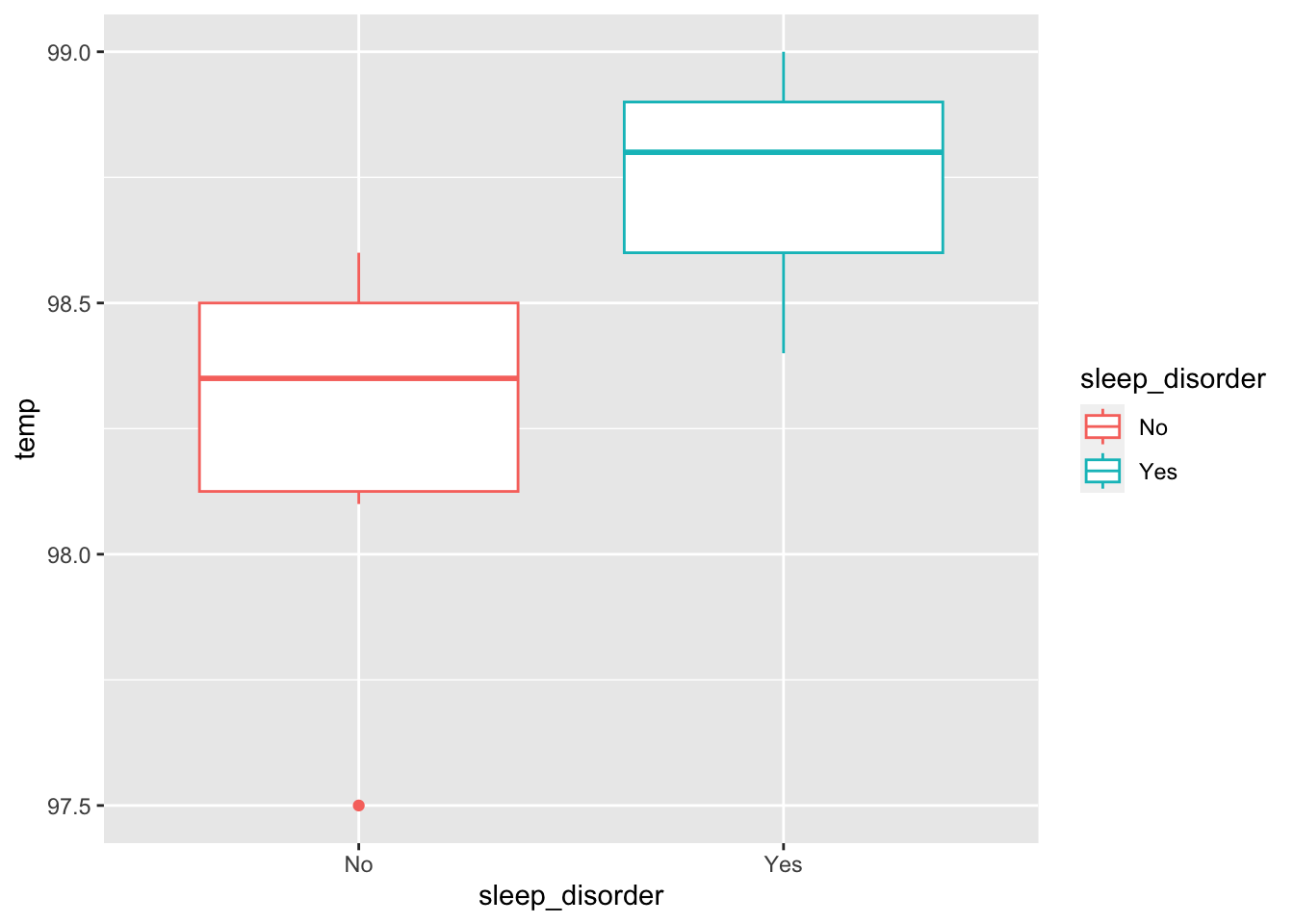
Ex 1

You are interested in determining if body temperature influences sleep disorder prevalence (yes 1, no 0). You collect the following trial data.

sleep_temp <- data.frame(
  temp = c(98.6, 98.5, 99, 97.5, 98.8, 98.2, 98.5, 98.4, 98.1), 
  sleep_disorder = c("No", "No", "Yes", "No", "Yes", "No", "No", "Yes", "No")
)
shapiro.test(sleep_temp$temp) # Normal

    Shapiro-Wilk normality test

data:  sleep_temp$temp
W = 0.94543, p-value = 0.6401
sleep_temp |> 
  ggplot(aes(sleep_disorder, temp, color = sleep_disorder)) +
  geom_boxplot()

  geom_point()
geom_point: na.rm = FALSE
stat_identity: na.rm = FALSE
position_identity 
wp.logistic(p0=0.33, p1=0.67, # Why ????
            alpha=0.05, power=0.80, 
            alternative="two.sided", family="normal")
Power for logistic regression

      p0   p1      beta0   beta1        n alpha power
    0.33 0.67 -0.7081851 1.41637 40.79646  0.05   0.8

URL: http://psychstat.org/logistic