Multi-class Performance Matrix

Pre-processing

set.seed(1)
iris_split <- initial_split(iris, prop = 0.7, strata = Species)
iris_tr <- training(iris_split)
iris_tst <- testing(iris_split)

Recipes

iris_rec <- recipe(Species ~ ., data = iris)

Model Spec

multinom_sim <- multinom_reg(engine = "nnet")

Workflow

iris_wf <- workflow(iris_rec, multinom_sim)

Fit & Predict

Fit Model

iris_fit <- fit(iris_wf, data = iris_tr)
iris_fit

══ Workflow [trained] ══════════════════════════════════════════════════════════
Preprocessor: Recipe
Model: multinom_reg()

── Preprocessor ────────────────────────────────────────────────────────────────
0 Recipe Steps

── Model ───────────────────────────────────────────────────────────────────────
Call:
nnet::multinom(formula = ..y ~ ., data = data, trace = FALSE)

Coefficients:
           (Intercept) Sepal.Length Sepal.Width Petal.Length Petal.Width
versicolor    53.35203     3.845927   -31.93694     10.02870   -3.275975
virginica    -57.85131   -23.541980   -41.71563     61.61759   31.272313

Residual Deviance: 0.1554973 
AIC: 20.1555

Predict

iris_res <- broom::augment(iris_fit, new_data = iris_tst)
head(iris_res)

# A tibble: 6 × 9
  Sepal.Length Sepal.Width Petal.Length Petal.Width Species .pred_class
         <dbl>       <dbl>        <dbl>       <dbl> <fct>   <fct>      
1          4.9         3            1.4         0.2 setosa  setosa     
2          5           3.6          1.4         0.2 setosa  setosa     
3          5.4         3.7          1.5         0.2 setosa  setosa     
4          4.8         3            1.4         0.1 setosa  setosa     
5          5.7         4.4          1.5         0.4 setosa  setosa     
6          5.4         3.9          1.3         0.4 setosa  setosa     
# ℹ 3 more variables: .pred_setosa <dbl>, .pred_versicolor <dbl>,
#   .pred_virginica <dbl>

Multi-class Performace Matrix

Confusion Matrix

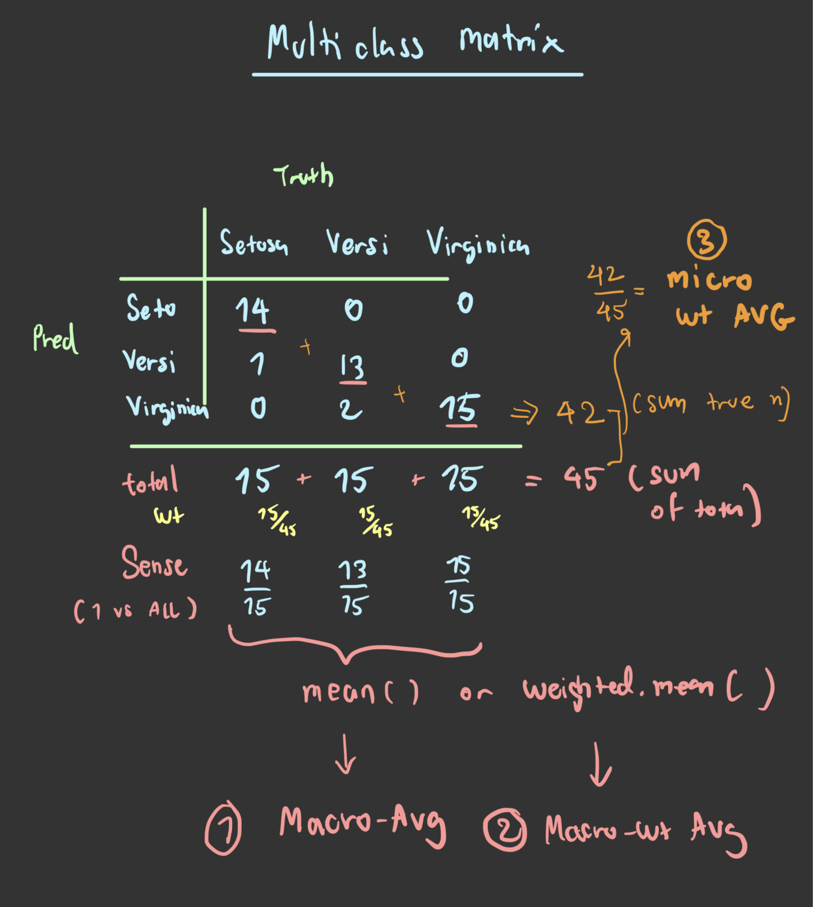
conf_mat(iris_res, truth = Species, estimate = .pred_class)

            Truth
Prediction   setosa versicolor virginica
  setosa         14          0         0
  versicolor      1         13         0
  virginica       0          2        15

Count number of observed class

class_totals <- iris_res |> 
  count(Species, name = "totals") %>% 
  mutate(class_wts = totals / sum(totals))

class_totals

# A tibble: 3 × 3
  Species    totals class_wts
  <fct>       <int>     <dbl>
1 setosa         15     0.333
2 versicolor     15     0.333
3 virginica      15     0.333

cell_counts <- 
  iris_res %>% 
  group_by(Species, .pred_class) %>% 
  count() %>% 
  ungroup()

cell_counts

# A tibble: 5 × 3
  Species    .pred_class     n
  <fct>      <fct>       <int>
1 setosa     setosa         14
2 setosa     versicolor      1
3 versicolor versicolor     13
4 versicolor virginica       2
5 virginica  virginica      15

# Compute the four sensitivities using 1-vs-all
one_versus_all <- 
  cell_counts %>% 
  filter(Species == .pred_class) %>% 
  full_join(class_totals, by = "Species") %>% 
  mutate(sens = n / totals)

one_versus_all

# A tibble: 3 × 6
  Species    .pred_class     n totals class_wts  sens
  <fct>      <fct>       <int>  <int>     <dbl> <dbl>
1 setosa     setosa         14     15     0.333 0.933
2 versicolor versicolor     13     15     0.333 0.867
3 virginica  virginica      15     15     0.333 1

# Three different estimates:
one_versus_all %>% 
  summarize(
    macro = mean(sens), 
    macro_wts = weighted.mean(sens, class_wts),
    micro = sum(n) / sum(totals)
  )

# A tibble: 1 × 3
  macro macro_wts micro
  <dbl>     <dbl> <dbl>
1 0.933     0.933 0.933

Macro-averaging: computes a set of one-versus-all metrics using the standard two-class statistics. These are averaged.
Macro-weighted averaging: does the same but the average is weighted by the number of samples in each class.
Micro-averaging: computes the contribution for each class, aggregates them, then computes a single metric from the aggregates.