library(infer)
library(dplyr)Infer Package Intro
I will explore {infer} Package.
Explore Data
glimpse(gss)
#> Rows: 500
#> Columns: 11
#> $ year    <dbl> 2014, 1994, 1998, 1996, 1994, 1996, 1990, 2016, 2000, 1998, 20…
#> $ age     <dbl> 36, 34, 24, 42, 31, 32, 48, 36, 30, 33, 21, 30, 38, 49, 25, 56…
#> $ sex     <fct> male, female, male, male, male, female, female, female, female…
#> $ college <fct> degree, no degree, degree, no degree, degree, no degree, no de…
#> $ partyid <fct> ind, rep, ind, ind, rep, rep, dem, ind, rep, dem, dem, ind, de…
#> $ hompop  <dbl> 3, 4, 1, 4, 2, 4, 2, 1, 5, 2, 4, 3, 4, 4, 2, 2, 3, 2, 1, 2, 5,…
#> $ hours   <dbl> 50, 31, 40, 40, 40, 53, 32, 20, 40, 40, 23, 52, 38, 72, 48, 40…
#> $ income  <ord> $25000 or more, $20000 - 24999, $25000 or more, $25000 or more…
#> $ class   <fct> middle class, working class, working class, working class, mid…
#> $ finrela <fct> below average, below average, below average, above average, ab…
#> $ weight  <dbl> 0.8960034, 1.0825000, 0.5501000, 1.0864000, 1.0825000, 1.08640…
Specifying Response specify()
Specify response and explanatory variable as formula or arguments.
Continuous Response
age (num) ~ partyid (fct)
gss_spec_age_partyid <- gss %>%
  specify(age ~ partyid)
#> Dropping unused factor levels DK from the supplied explanatory variable 'partyid'.

# Object Type
sloop::otype(gss_spec_age_partyid)
#> [1] "S3"
# Class
class(gss_spec_age_partyid)
#> [1] "infer"      "tbl_df"     "tbl"        "data.frame"
# Print
gss_spec_age_partyid
#> Response: age (numeric)
#> Explanatory: partyid (factor)
#> # A tibble: 500 × 2
#>      age partyid
#>    <dbl> <fct>
#>  1    36 ind
#>  2    34 rep
#>  3    24 ind
#>  4    42 ind
#>  5    31 rep
#>  6    32 rep
#>  7    48 dem
#>  8    36 ind
#>  9    30 rep
#> 10    33 dem
#> # … with 490 more rows
Categorical Response
specifying for inference on proportions
you will need to use the success argument to specify which level of your response variable is a success.
gss %>%
  specify(response = college, success = "degree")
#> Response: college (factor)
#> # A tibble: 500 × 1
#>    college
#>    <fct>
#>  1 degree
#>  2 no degree
#>  3 degree
#>  4 no degree
#>  5 degree
#>  6 no degree
#>  7 no degree
#>  8 degree
#>  9 degree
#> 10 no degree
#> # … with 490 more rows
Declare the NULL Hypothesis
declare a null hypothesis using hypothesize().
null: “independence” or “point”.
Test Independence
If the null hypothesis is that the mean number of hours worked per week in our population is 40, we would write:
gss %>%
  specify(college ~ partyid, success = "degree") %>%
  hypothesize(null = "independence")
#> Dropping unused factor levels DK from the supplied explanatory variable 'partyid'.
#> Response: college (factor)
#> Explanatory: partyid (factor)
#> Null Hypothesis: independence
#> # A tibble: 500 × 2
#>    college   partyid
#>    <fct>     <fct>
#>  1 degree    ind
#>  2 no degree rep
#>  3 degree    ind
#>  4 no degree ind
#>  5 degree    rep
#>  6 no degree rep
#>  7 no degree dem
#>  8 degree    ind
#>  9 degree    rep
#> 10 no degree dem
#> # … with 490 more rows
Test Point Estimate
gss %>%
  specify(response = hours) %>%
  hypothesize(null = "point", mu = 40)
#> Response: hours (numeric)
#> Null Hypothesis: point
#> # A tibble: 500 × 1
#>    hours
#>    <dbl>
#>  1    50
#>  2    31
#>  3    40
#>  4    40
#>  5    40
#>  6    53
#>  7    32
#>  8    20
#>  9    40
#> 10    40
#> # … with 490 more rows
generate() NULL distribution
set.seed(1)

gss %>%
  specify(response = hours) %>%
  hypothesize(null = "point", mu = 40) %>%
  generate(reps = 1000, type = "bootstrap")
#> Response: hours (numeric)
#> Null Hypothesis: point
#> # A tibble: 500,000 × 2
#> # Groups:   replicate [1,000]
#>    replicate hours
#>        <int> <dbl>
#>  1         1 46.6
#>  2         1 43.6
#>  3         1 38.6
#>  4         1 28.6
#>  5         1 38.6
#>  6         1 38.6
#>  7         1  6.62
#>  8         1 78.6
#>  9         1 38.6
#> 10         1 38.6
#> # … with 499,990 more rows
Calculate Summary Stats
find the point estimate
obs_mean <- gss %>%
  specify(response = hours) %>%
  calculate(stat = "mean")

obs_mean
#> Response: hours (numeric)
#> # A tibble: 1 × 1
#>    stat
#>   <dbl>
#> 1  41.4
generate a null distribution
null_dist <- gss %>%
  specify(response = hours) %>%
  hypothesize(null = "point", mu = 40) %>%
  generate(reps = 1000, type = "bootstrap") %>%
  calculate(stat = "mean")

null_dist
#> Response: hours (numeric)
#> Null Hypothesis: point
#> # A tibble: 1,000 × 2
#>    replicate  stat
#>        <int> <dbl>
#>  1         1  40.5
#>  2         2  40.1
#>  3         3  39.1
#>  4         4  40.3
#>  5         5  38.8
#>  6         6  39.6
#>  7         7  40.2
#>  8         8  40.4
#>  9         9  40.1
#> 10        10  40.6
#> # … with 990 more rows
Visualize Null Dist
null_dist %>%
  visualize()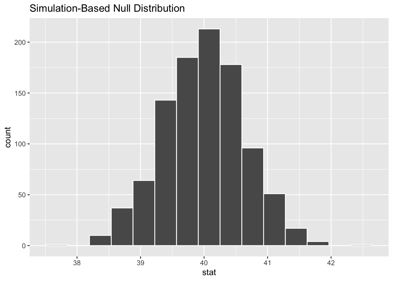
Where does our sample’s observed statistic lie on this distribution? We can use the obs_stat argument to specify this.
null_dist %>%
  visualize() +
  shade_p_value(obs_stat = obs_mean, direction = "two-sided")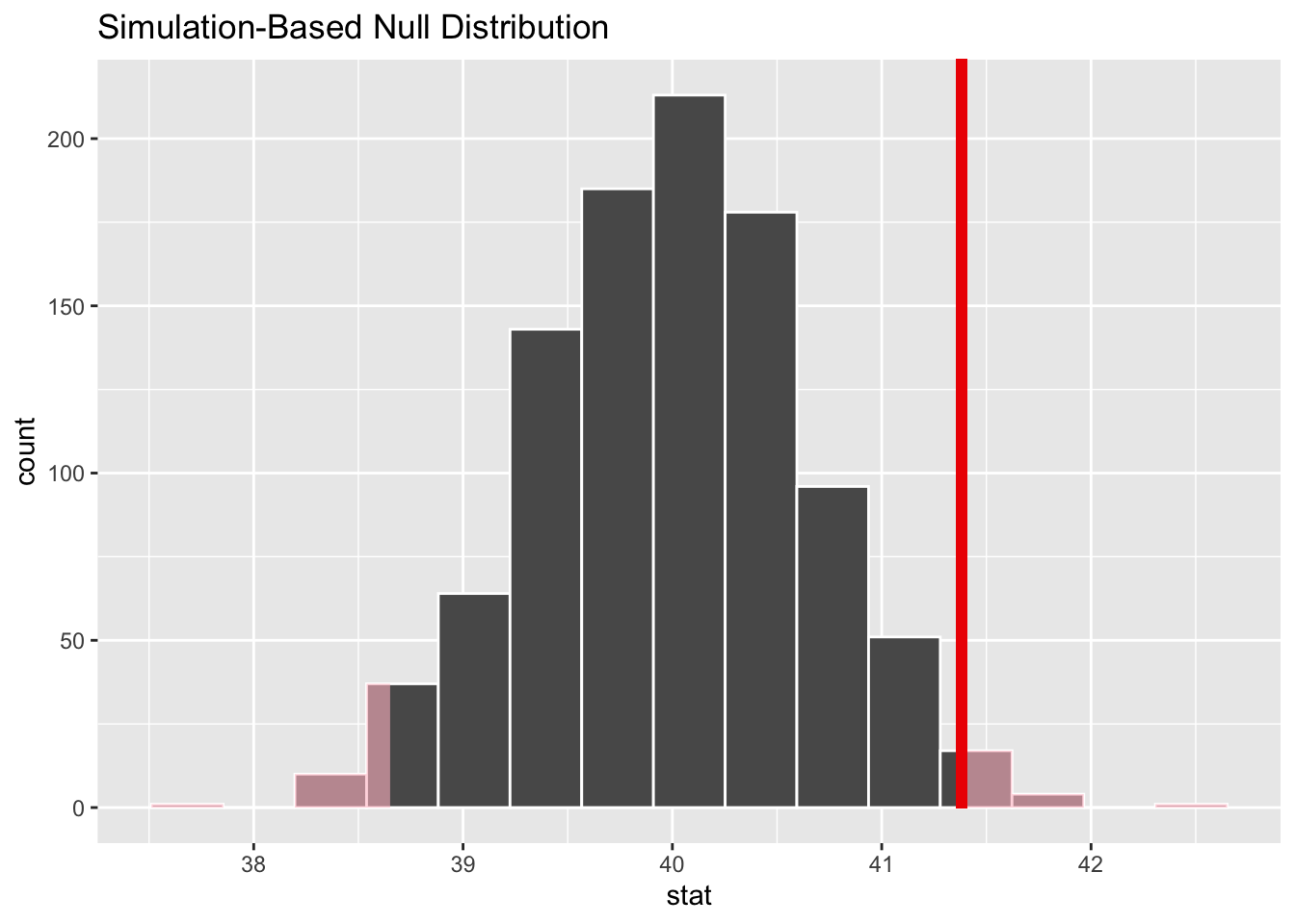
P-value
get a two-tailed p-value
p_value <- null_dist %>%
get_p_value(obs_stat = obs_mean, direction = "two-sided")
p_value
#> # A tibble: 1 × 1
#> p_value
#> <dbl>
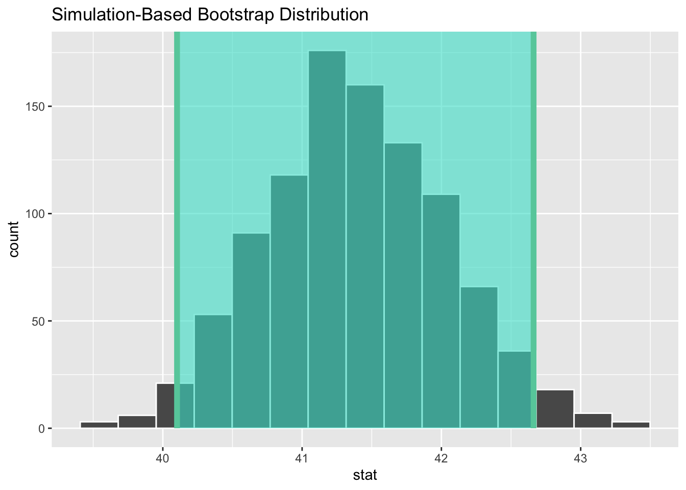
#> 1 0.038Confidence Interval
# generate a distribution like the null distribution,
# though exclude the null hypothesis from the pipeline
boot_dist <- gss %>%
  specify(response = hours) %>%
  generate(reps = 1000, type = "bootstrap") %>%
  calculate(stat = "mean")

# start with the bootstrap distribution
ci <- boot_dist %>%
  # calculate the confidence interval around the point estimate
  get_confidence_interval(point_estimate = obs_mean,
                          # at the 95% confidence level
                          level = .95,
                          # using the standard error
                          type = "se")

ci
#> # A tibble: 1 × 2
#>   lower_ci upper_ci
#>      <dbl>    <dbl>
#> 1     40.1     42.7
boot_dist %>%
visualize() +
shade_confidence_interval(endpoints = ci)