library(pwr)
library(WebPower)
library(simstudy)Sample Size (2)
Adapted from these sources:
Overview
Typical Values
A two-tailed test
a significance of 0.05 and a power of 80% was established.
For nonparametric tests on continuous variables, as a rule of thumb, calculate the sample size required for parametric tests and add 15%
Effect Size
Effect size can be defined as ‘a standardized measure of the magnitude of the mean difference or relationship between study groups’
An index that divides the effect size by its dispersion (standard deviation, etc.) is not affected by the measurement unit and can be used regardless of the unit, and is called an ‘effect size index’ or ’standardized effect size
Whether an effect size should be interpreted as small, medium, or large may depend on the analysis method.
We use the guidelines mentioned by Cohen and Sawilowsky and use the medium effect size considered for each test in the examples below.
Conventional Effect Size
cohen.ES(test = "t", size = "medium")
     Conventional effect size from Cohen (1982)

           test = t
           size = medium
    effect.size = 0.5
Dropout Rate
If dr is the dropout rate,
N = n / (1 – dr)
Continuous outcome of 2 groups
pwr.t.test() function
- one-sample t test (type = “one.sample”)
- two-sample t test (type = “two.sample”)
- paired t test (type = “paired”).
Cohen’s d is used as the effect size
- Very small (d = 0.01)
- Small (d = 0.2)
- Medium (d = 0.5)
- Large (d = 0.8)
- Very large (d = 1.2)
- Huge (d = 2)
In our example, we will use medium effect size (d = 0.5).
One-sample t-test
Cohen’s d:
\[ d = \frac{\mu_1 - \mu_0}{SD} \]
Where:
- \(\mu_0\) = mean under \(H_0\)
- \(\mu_1\) = mean under \(H_1\)
- \(SD\) = SD under \(H_0\)
Ex 1
pwr.t.test(d = 0.5, sig.level = 0.05, power = 0.8, type = "one.sample", alternative = "two.sided")
     One-sample t test power calculation

              n = 33.36713
              d = 0.5
      sig.level = 0.05
          power = 0.8
    alternative = two.sided
N = 34 (If dropout rate of 20%, a total of 43 samples are required)
Ex 2: New DM Drug
Let’s propose a study of a new drug to reduce hemoglobin A1c in type 2 diabetes over a 1 year study period. You estimate that your recruited participants will have a mean baseline A1c of 9.0, which will be unchanged by your placebo, but reduced (on average) to 7.0 by the study drug.
let’s say 5.0 and 17.0 for min and max of Hgb A1c
sd_approx <- (17 - 5)/4
d1 <- (9 - 7) / sd_approx # delta / sd

pwr::pwr.t.test(n = NULL,
                sig.level = 0.05,
                type = "two.sample",
                alternative = "two.sided",
                power = 0.80,
                d = d1)
     Two-sample t test power calculation

              n = 36.30569
              d = 0.6666667
      sig.level = 0.05
          power = 0.8
    alternative = two.sided

NOTE: n is number in *each* group
N = 37 in each group (Assuming a 20% dropout rate in each arm, would require 37*5/4 subjects per arm)
If study on 50 participants, what would the power be?
pwr::pwr.t.test(n = 25, # note that n is per arm
                sig.level = 0.05,
                type = "two.sample",
                alternative = "two.sided",
                power = NULL, # ?
                d = 0.66)
     Two-sample t test power calculation

              n = 25
              d = 0.66
      sig.level = 0.05
          power = 0.6280322
    alternative = two.sided

NOTE: n is number in *each* group
Two-sample t-test
Cohen’s d for Welch:
\[ d = \frac{ \mu_1 - \mu_2 }{SD_{pool}} \]
Where
\[ SD_{pool} = \sqrt{ (SD_1^2 + SD_2^2)/2 } \]
pwr.t.test(d = 0.5, sig.level = 0.05, power = 0.8,
           type = "two.sample",
           alternative = "two.sided")
     Two-sample t test power calculation

              n = 63.76561
              d = 0.5
      sig.level = 0.05
          power = 0.8
    alternative = two.sided

NOTE: n is number in *each* group
Assuming a p-value of 0.05 and a power of 80% in a two-tailed test, when the effect size d = 0.5
N = 64 x 2 (dropout rate of 20%, Total = 160)
Paired t-test
pwr.t.test(d = 0.5, sig.level = 0.05, power = 0.8,
           type = "paired",
           alternative = "two.sided")
     Paired t test power calculation

              n = 33.36713
              d = 0.5
      sig.level = 0.05
          power = 0.8
    alternative = two.sided

NOTE: n is number of *pairs*
Assuming a p-value of 0.05 and a power of 80% in a two-tailed test, the minimum number of pairs required to demonstrate statistical signifi- cance is 34 when the effect size d = 0.5.
Considering the dropout rate of 20%, a total of 43 pairs are required.
Non-parametric
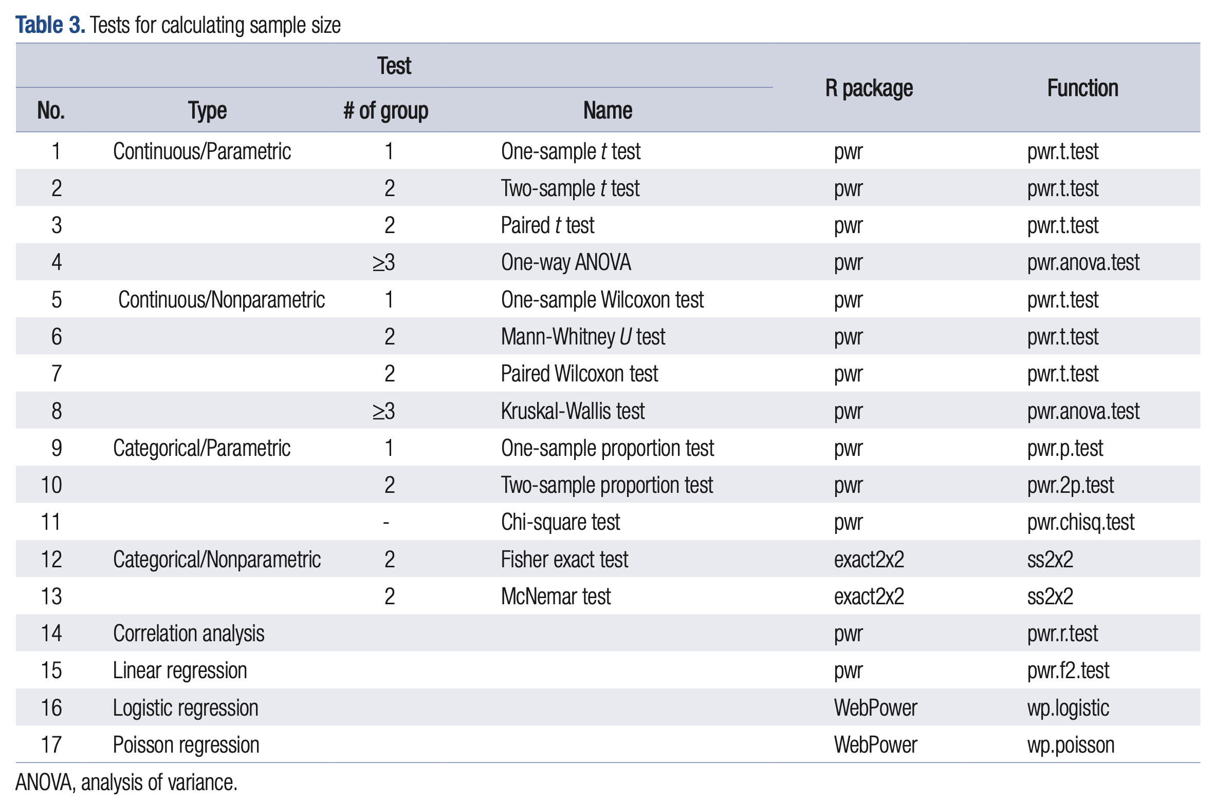
One-sample Wilcoxon test (Table 3, no. 5)
A total of 43 was calculated by one-sample t test and adding 15% gives a total of 65.
Mann-Whitney U test (Table 3, no. 6)
By two-sample t test, 80 people were calculated for each group, and a total of 240 people was calculated by considering an addi- tional 15% for each group.
Paired Wilcoxon test (Table 3, no. 7)
The 43 pairs were calculated by paired t test, taking into ac- count an additional 15%, the total 65 pairs are required.
Continuous outcome of ≥3 groups
ANOVA (Parametric)
Studies that compare averages of three or more groups.
k: number of comparison groupsf: means the effect size (Cohen’s \(f\))
\[ f = \sqrt{ \frac{ \sum_{i=1}^{k} p_i \times (\mu_i - \mu)^2 }{\sigma^2} } \]
Effect Size (f-values)
- Small = 0.1
- Medium = 0.25
- Large = 0.4
cohen.ES(test = "anov", size = "medium")
     Conventional effect size from Cohen (1982)

           test = anov
           size = medium
    effect.size = 0.25
pwr.anova.test (k = 3 , f = 0.25, sig.level = 0.05, power = 0.8)
     Balanced one-way analysis of variance power calculation

              k = 3
              n = 52.3966
              f = 0.25
      sig.level = 0.05
          power = 0.8

NOTE: n is number in each group
Assume that the p-value is 0.05, the power is 80%, and the two-tailed test is performed. When the total comparison group was three groups and the effect size value was 0.25, the number of subjects calculated was 53 in each group.
Considering a dropout rate of 20%, a total of 198 samples are required, which is calculated as 66 per group.
Kruskal-Wallis test (Non-parametric)
By one-way ANOVA, 66 people were calculated for each group, and if 15% of each group is additionally considered, a total of 297 people are calculated.
Proprotion
Effect Size
Cohen’s h
\[ h = 2 \times asin(\sqrt{p_1})-2 \times asin(\sqrt{p_2}) \] h-values
- Small = 0.2
- Medium = 0.5
- Large = 0.8
One-sample proportion test
Let’s assume that patients discharged from your hospital after a myocardial infarction have historically received a prescription for aspirin 80% of the time. A nursing quality improvement project on the cardiac floor has tried to increase this rate to 95%. How many patients do you need to track after the QI intervention to determine if the proportion has truly increased?
the null hypothesis is that the proportion is 0.8
the alternative hypothesis is that the proportion is 0.95.
Effect size (Cohen’s h):
ES.h(p1 = 0.95, p2 = 0.80)[1] 0.4762684pwr.p.test(h = ES.h(p1 = 0.95, p2 = 0.80),
n = NULL,
sig.level = 0.05,
power = 0.80,
alternative = "greater")
     proportion power calculation for binomial distribution (arcsine transformation)

              h = 0.4762684
              n = 27.25616
      sig.level = 0.05
          power = 0.8
    alternative = greater
Two-sample proportion test (equal n)
You want to calculate the sample size for a study of a cardiac plexus parasympathetic nerve stimulator for pulmonary hypertension. You expect the baseline one year mortality to be 15% in high-risk patients, and expect to reduce this to 5% with this intervention. You will compare a sham (turned off) stimulator to an active stimulator in a 2 arm study. Use a 2-sided alpha of 0.05 and a power of 80%.
Effect size (Cohen’s h):
ES.h(p1 = 0.15, p2 = 0.05)[1] 0.344372pwr.p.test(h = ES.h(p1 = 0.15, p2 = 0.05),
n = NULL,
sig.level = 0.05,
power = 0.80,
alternative = "two.sided")
     proportion power calculation for binomial distribution (arcsine transformation)

              h = 0.344372
              n = 66.18368
      sig.level = 0.05
          power = 0.8
    alternative = two.sided
We need to enroll at least 67 per arm, or 134 overall.
Two-sample proportion test (unequal n)
Imagine you want to enroll class IV CHF patients in a device trial in which they will be randomized 3:1 to a device (vs sham) that restores their serum sodium to 140 mmol/L and their albumin to 40 mg/dL each night. You expect to reduce 1 year mortality from 15% to 5% with this device. You want to know what your power will be if you enroll 300 in the device arm and 100 in the sham arm.
pwr.2p2n.test(h = ES.h(p1 = 0.15, p2 = 0.05),
              n1 = 300,
              n2 = 100,
              sig.level = 0.05,
              power = NULL,
              alternative = "two.sided")
     difference of proportion power calculation for binomial distribution (arcsine transformation)

              h = 0.344372
             n1 = 300
             n2 = 100
      sig.level = 0.05
          power = 0.8467011
    alternative = two.sided

NOTE: different sample sizes
This (300:100) enrollment will have 84.6% power to detect a change from 15% to 5% mortality, with a two-sided alpha of 0.05.